
ENG - Machine Learning based Predictive Maintenance - Part 3 : The modeling part
The Pharm'AI Company - Project #5

After completing the analysis of a real dataset together, it’s now time to move on to the third and final step: training a Machine Learning model to create a predictive tool that turns data into action!
The application prototype is available here.
Redefining the Problem
Let’s recap some key points from the second article to quickly recontextualize the problem from a “Data” perspective.
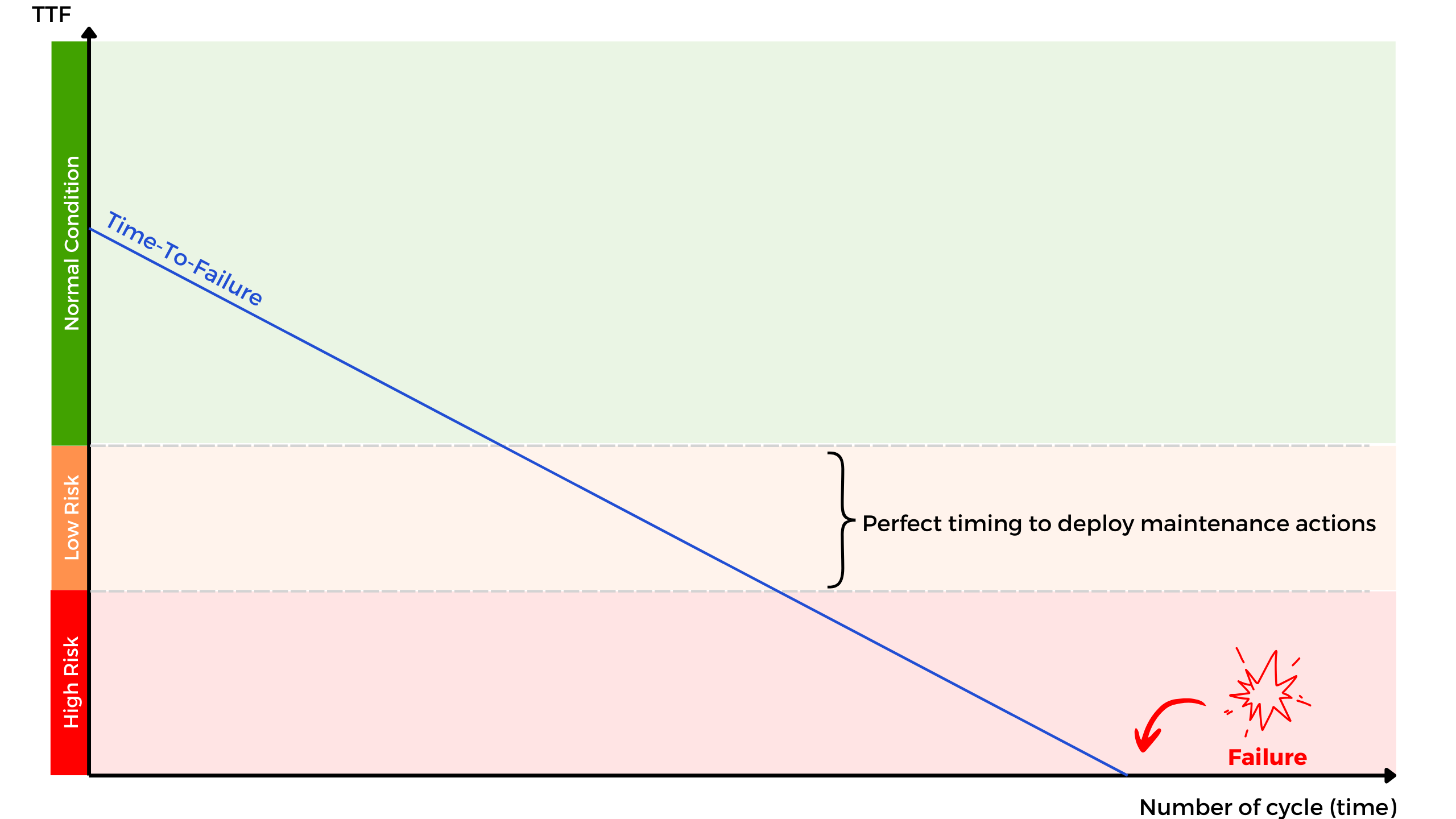
We monitored a hundred turbines over an extended period. This monitoring allowed us to collect numerical readings from over twenty sensors (temperature, pressure, vibrations, etc.), as well as an assessment of failure risk through the TTF (Time-To-Failure).
The goal of our model is to predict the risk level of failure based on new input data, assigning it to one of the following three categories:
Class 0: Normal operation (no risk)
Class 1: Caution zone (moderate risk, maintenance recommended)
Class 2: Critical zone (high risk of imminent failure)
In terms of modeling, the task is to predict one of three categories. In Data Science, this is referred to as a multi-class classification problem.
From an operational perspective, the most critical category for us is Class 1, as this is the ideal moment to trigger maintenance actions.
Choosing the Right Algorithm
It’s often challenging to determine in advance which algorithm will best suit a given problem. There’s no universal algorithm that outperforms all others in every scenario. In Machine Learning, this reality is well encapsulated by the theorem formulated by David Wolpert, famously known as the “No Free Lunch” theorem1.
There is no free lunch! — David Wolpert
This principle underscores that no algorithm is optimal for every problem; each tool has its strengths and weaknesses depending on the context.
During the development phase, it’s common to evaluate multiple algorithms in parallel to choose the one offering the best trade-offs based on the project’s criteria. These criteria include prediction quality, model explainability, inference time, and even energy consumption.
To simplify this project and avoid unnecessary complexity, I opted not to compare a range of algorithms but instead to focus directly on a specific method, i.e. Random Forest2.
This algorithm typically provides a good balance between performance and computational efficiency.

For a detailed explanation of how decision-tree-based algorithms work—particularly Random Forest—please refer to the link and video3 below.
Training the Model
Training a Machine Learning algorithm involves several strategic steps to ensure the reliability of our predictions. Below is a summary of these steps, but the full code is, of course, available in this notebook4.
Step #1: Data Preparation
Our initial dataset shows a marked imbalance: 17,531 observations correspond to normal operation, while only around 1,500 observations each represent moderate and high-risk states. This is quite logical—machines are more often in good working condition than close to failure.
To address this imbalance, which could bias our model, I used a statistical technique called SMOTE, which generates synthetic examples to balance the classes. Sensor measurements were also standardized (NB: Standardization is unnecessary for tree-based approaches like Random Forest but is essential for methods like PCA).
Step #2: Creating a Performance Metric
By definition, an algorithm will make prediction errors; a 100% accurate model doesn’t exist. For this project, I wanted to minimize prediction errors in Class 1 at all costs, as this category triggers maintenance actions.
The choice of performance metric is crucial because it directly influences and guides the training phase. I developed a custom performance metric (recall * 0.7 + accuracy * 0.3) that penalizes misclassifications in Class 1 more heavily.
This strategy does lead to some false positives, resulting in slightly excessive maintenance actions. However, this approach aligns with the project’s priority: avoiding missed opportunities for preventive maintenance.
Step #3: Training the Model
As with all algorithms, the model training phase involves various optimization processes to converge toward the optimal parameters for the Random Forest model.
A brief technical explanation for Data Science enthusiasts (apologies to the uninitiated 🤯):
Hyperparameter optimization was conducted using GridSearchCV, which tests different combinations of parameters, including:
Tree depth (from 4 to 8 levels),
Splitting criteria (Gini or entropy),
Minimum number of samples per split.
A classic train/test split approach combined with 5-fold cross-validation and random permutations ensures robust results.
Step #4: Performance Evaluation
The results are promising: our model achieves 87% recall for detecting turbines in Class 1 and, most importantly, misses no critical Class 2 cases. Although the model can be overly cautious, misclassifying compliant turbines as risky, this trade-off is acceptable in a safety-first context.
Detection isn’t perfect, but that’s not a major concern. Class 1 spans about twenty cycles, making it nearly impossible to overlook a machine entering the red zone.
The only potential risks are encountering a new failure mode not captured during training or a sudden, unexpected breakdown.
Conclusion
An analysis of the most influential sensors reveals the critical importance of:
Sensors s7 and s11 (measuring compressor discharge pressure),
Sensor s4 (monitoring the low-pressure turbine outlet temperature),
Sensor s12 (tracking the fuel flow ratio).

These sensors play a key role in our model’s predictions. Beyond modeling, it would be beneficial to incorporate these measurements into reference documentation and training programs as “sentinels” for monitoring equipment health.
From Prototype to Production
Solution Architecture
Transitioning from a prototype to an operational solution often represents a major challenge in data science projects. To make the model accessible and usable, I opted for a simple yet effective architecture based on an interactive web application developed with Streamlit5 (NB: I’ve previously discussed this framework in earlier projects).
Webapp overview
The user interface developed with Streamlit includes the following features:
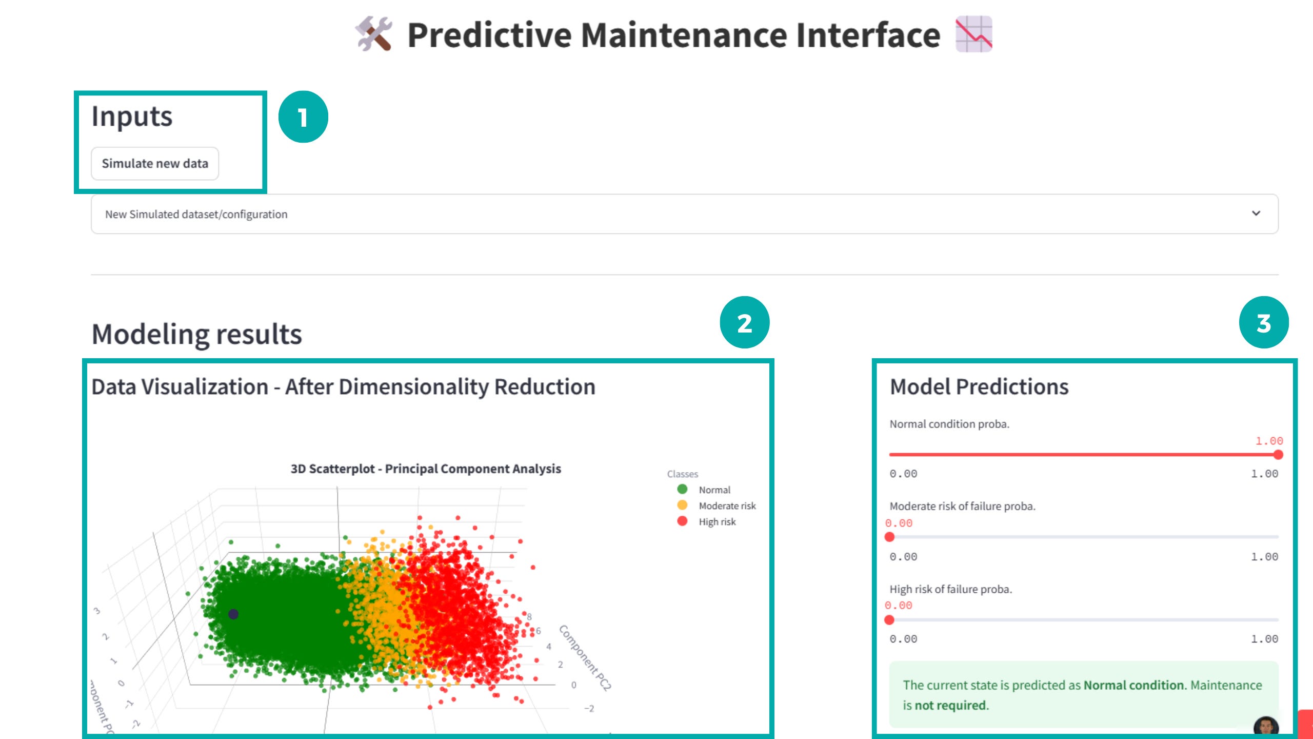
Simulating new sensor data:
A button generates random new configurations of values outside the training dataset.
3D Visualization of Results:
A PCA-based visualization shows the machine’s new state relative to historical data.
Prediction Panel:
For each new configuration, the app displays the probabilities for each risk level, along with clear maintenance action recommendations.
Potential Improvements
Real-Time Integration
The data used for this project was batch-collected. However, real-time sensor data is becoming the standard for such applications. This would involve:
Ingesting continuous data streams.
Preprocessing signals to reduce noise in input data.
Using Deep Learning algorithms capable of detecting anomalies in time series, coupled with an automatic alert system.
This predictive maintenance project clearly calls for a follow-up project with continuous data. (NB: This is on my to-do list 😃!)
Enriching the Dataset
The tool we’ve created is purely mathematical, based solely on sensor data. However, we could build more sophisticated tools by combining raw data with:
CMMS data (Computerized Maintenance Management System—detailed intervention history),
Functional analyses of equipment,
Incident reports and failure descriptions,
Maintenance technicians’ and engineers’ expertise,
...and more.
This would enable predictions not only of failure risk but also failure modes, root causes, and priority corrective actions, resulting in a much smarter tool capable of guiding the type and content of predictive maintenance interventions.
Advanced Monitoring System
The model was built using data from a single collection campaign. However, machines are dynamic systems, and we likely didn’t capture their full complexity during an isolated measurement campaign. A predictive tool valid at a specific time may quickly become obsolete.
To address this, it’s crucial to implement a data collection system paired with performance monitoring to retrain the model regularly, if needed.
Conclusion
We’ve just explored, step by step, the deployment of a Machine Learning project in an industrial context. This project, though educational and intentionally simplified, highlights the many technical and strategic challenges of creating a predictive maintenance solution.
To go further, initiatives such as integrating continuous data or leveraging CMMS databases could not only enhance precision but also provide deeper insights into failure modes and prioritize interventions.
Feel free to share your feedback and experiences in the comments!
… Let’s rock with data! 🤘